Can an electric-field trace reveal a plasma’s density? This small JAX example connects a fluid simulation to a synthetic measurement and uses automatic differentiation to estimate the density.
Download code, notebook, and results (ZIP) · Browse on GitHub
Watch the plasma oscillate
A small electron-density perturbation creates an electric field. The restoring force drives an oscillation while the ions remain fixed. The animation follows one period in a periodic, one-centimeter domain.
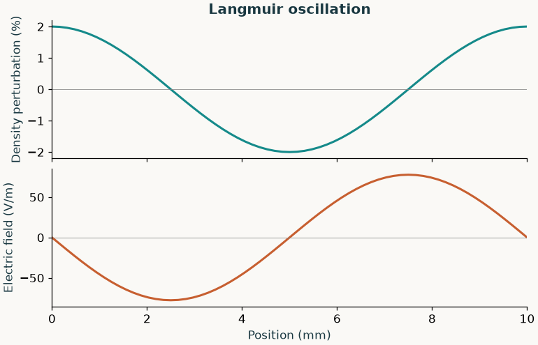
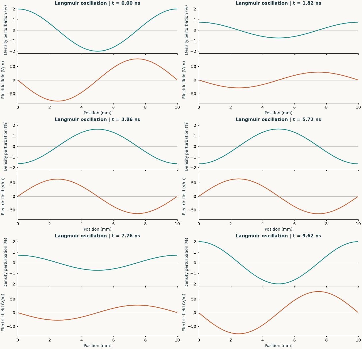
This is a linear cold-electron fluid model with a 2% initial density perturbation. It resolves density, velocity, and the self-consistent electric field on a grid. It does not include electron temperature, collisions, ion motion, or kinetic effects such as Landau damping.
From a measurement to a density
The synthetic plasma has a density of 1.35 × 10¹⁴ m⁻³. Starting from 1.00 × 10¹⁴ m⁻³, the optimizer adjusts the density to match an electric-field trace at one location. JAX calculates the derivatives through the numerical time steps and Poisson solves.
The observations come from the independent analytical solution. The noisy case adds Gaussian noise with a standard deviation equal to 3% of the initial field peak. Both fits use 181 samples over about 32 nanoseconds.
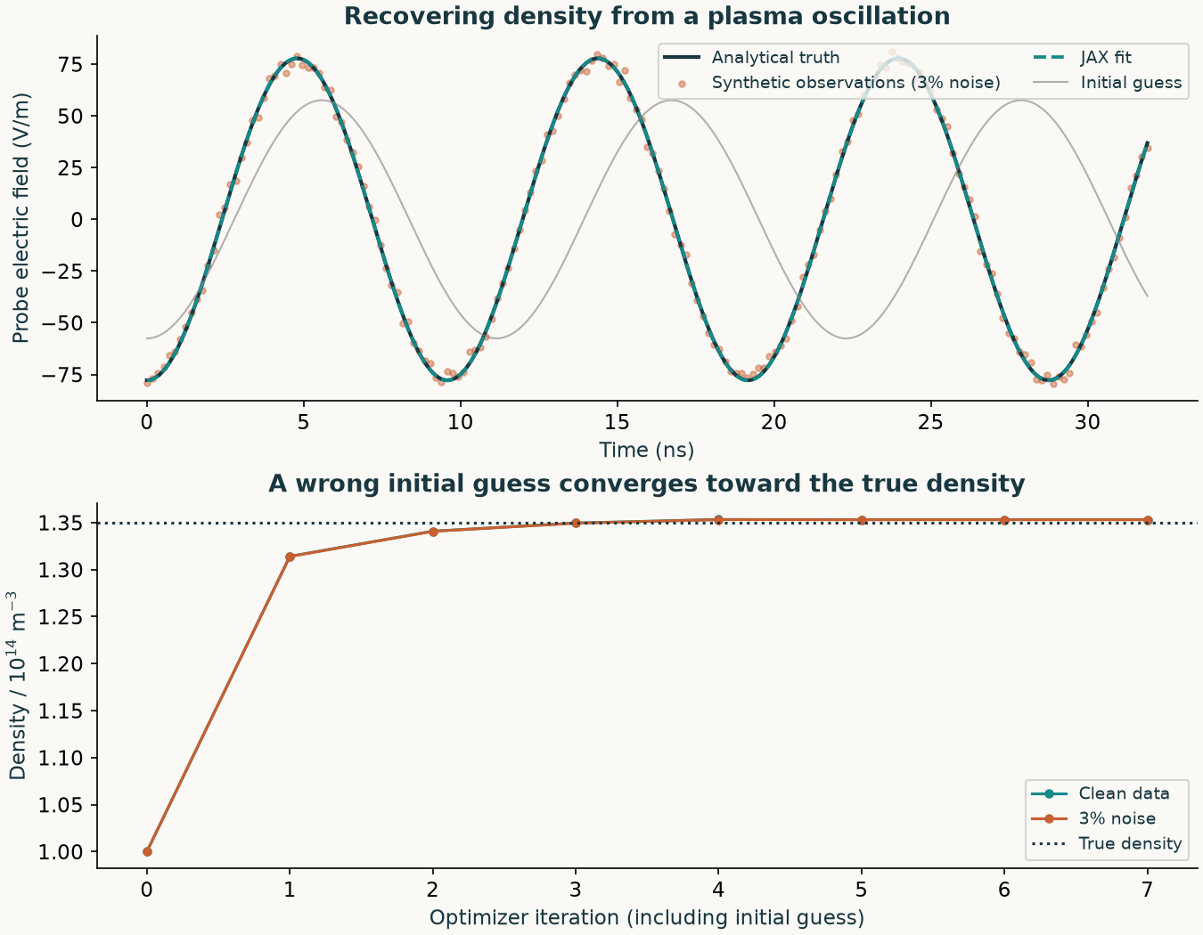
Top: analytical truth, synthetic observations, initial guess, and fitted trace. Bottom: density updates during optimization. Click to enlarge.
| Experiment | Recovered density (10¹⁴ m⁻³) | Relative error |
|---|---|---|
| Clean data, 64 points | 1.35321 | +0.238% |
| 3% noise, 64 points | 1.35309 | +0.229% |
| Clean data, 128 points | 1.35080 | +0.0594% |
Doubling the grid resolution reduces the clean-data bias by approximately fourfold. The noisy result is one reproducible realization, not an uncertainty bound. The experiment assumes a known initial perturbation, phase, probe position, and measurement calibration; only density is fitted.
What changes in space and time?
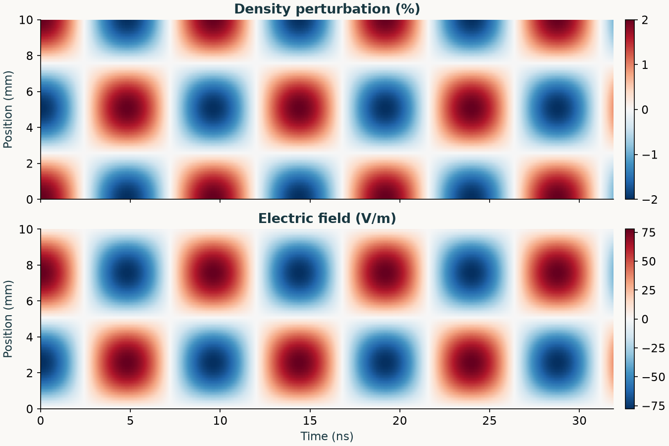
Density and electric-field evolution at the true density. Color scales remain fixed throughout the run.
Validation, not just a fit
The code is checked against the analytical plasma frequency and field trace, and against finite-difference derivatives. All reported calculations ran on a CPU using 64-bit arithmetic.
- Frequency: 0.120% error on 64 grid points, decreasing to 0.0301% on 128 points.
- Spatial convergence: approximately second order against the analytical continuum solution.
- Time integration: approximately fourth order against the exact spatially discretized solution.
- Gradients: relative discrepancies below 10⁻⁸ in the finest finite-difference check at three trial densities.
- Consistency: equilibrium, charge neutrality, and the discrete Poisson equation pass; maximum relative discrete-energy drift is about 6 × 10⁻⁹ in the demonstration run.
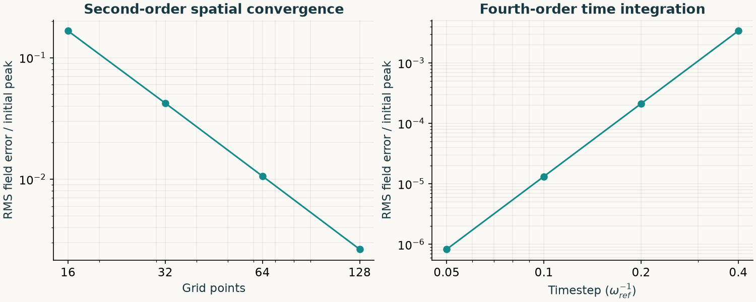
Separate checks isolate spatial and temporal errors. The README defines the reference solutions and discrete energy.
The solver uses centered finite differences, an FFT inversion of the discrete Poisson operator, and fourth-order Runge–Kutta time stepping. Reference units stay fixed during inference, preserving the density dependence of the physical oscillation frequency. These tests validate the documented small-amplitude example, not arbitrary plasma conditions or a complete discharge model.
Run and explore
Tested with Python 3.12. From the extracted langmuir-jax folder, preferably in a virtual environment:
python -m pip install -r requirements.txt
python run_example.py --check-only
python run_example.py --output results
Open explore.ipynb for a short notebook introduction. The download includes the solver, inference and validation driver, pinned dependencies, all figures, the animation, CSV traces, field arrays, and a JSON summary. A GPU is not required.